cs231n assignment1(Two_Layer_Net)
两层网络(code)
首先来回顾一下我们的网络结结构:
输入层($D$个神经元),全连接层-ReLu($H$),softmax($C$)。
输入:$X [N\times{D}]$,输出 $y [N\times{1}]$
网络参数:$W1[D×H],b1[1×H],W2[H×C],b2[1×C]$
Propagation
$Z2 \color{Blue}{[N\times{C}]}$就是每个样本在每个类别下的分数(score)
$A2 \color{Blue}{[N\times{C}]}$就是每个样本在每个类别下的概率(prob)
关键代码如下:
(Propagation中计算的值,Backpropogation的计算中要用到)1
2
3
4
5
6
7Z1 = np.dot(X, W1) + b1
A1 = np.maximum(0, Z1)
Z2 = np.dot(A1, W2) + b2
scores = Z2
scores -= np.max(scores, axis=1, keepdims=True)
A2 = np.exp(scores) / np.sum(np.exp(scores), axis=1, keepdims=True)
prob = A2
loss
关键代码如下:1
2
3
4# 最大似然项
loss += -np.sum(np.log(prob[(range(N), y)])) / N
# 正则化项
loss += reg * (np.sum(W1 * W1) + np.sum(W2 * W2))
Backpropogation
反向传播的推导,主要还是依据链式法则,从后至前进行推导。
MaskMat参见softmax_no_loop梯度推导
关键代码:1
2
3
4
5
6
7
8
9
10
11
12
13
14
15
16# softmax函数求导
prob[(range(N), y)] -= 1
dZ2 = prob / N
dW2 = np.dot(A1.T, dZ2)
db2 = np.ones((1, A1.shape[0])).dot(dZ2)
dA1 = dZ2.dot(W2.T)
dZ1 = dA1.copy()
dZ1[A1 <= 0] = 0
dW1 = X.T.dot(dZ1)
db1 = np.ones((1, N)).dot(dZ1)
# regulation
dW1 += 2 * reg * W1
dW2 += 2 * reg * W2
训练
train函数
还是采用stochastic gradient descent (SGD)进行优化。
具体操作与前面的线性学习器相同。每次迭代随机一小部分样本进行梯度下降:1
2
3
4
5for it in range(num_iters):
index = np.random.choice(num_train, batch_size)
X_batch = X[index]
y_batch = y[index]
...
值得一提的是,随着优化的进行,我们离最小点越来越近,所以希望learning rate也越来越小,这样更可能不错过最小点的位置。
所以设置一个decay rate,每次Echo后与学习率相乘,使其相应变小。1
2
3
4
5
iterations_per_epoch = max(num_train / batch_size, 1)
# Every epoch, decay learning rate.
if it % iterations_per_epoch == 0:
    learning_rate *= learning_rate_decay
train a network
先用默认的参数,训练一个网络1
2
3
4
5
6
7
8
9
10
11
12
13
14input_size = 32 * 32 * 3
hidden_size = 50
num_classes = 10
net = TwoLayerNet(input_size, hidden_size, num_classes)
# Train the network
stats = net.train(X_train, y_train, X_val, y_val,
num_iters=1000, batch_size=200,
learning_rate=1e-4, learning_rate_decay=0.95,
reg=0.25, verbose=True)
# Predict on the validation set
val_acc = (net.predict(X_val) == y_val).mean()
print('Validation accuracy: ', val_acc)
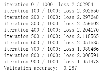
debug the training
可以看到我们用默认参数训练出的模型只有0.287的准确度。
一种方法就是,画出优化中损失函数和准确度的变化(可能每隔100次梯度下降就记录一下,然后画出来),找一下问题。
1 | # Plot the loss function and train / validation accuracies |
代码中的loss_history、train_acc_history、val_acc_history都是在模型训练中,每隔100次迭代记录下来的。目的就是为了这时候,可以将梯度下降的过程可视化。
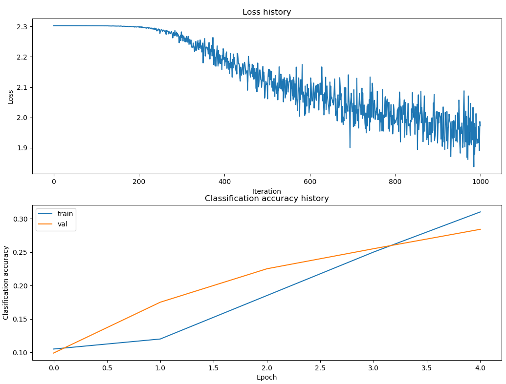
- 损失曲线下降趋势有点直,问题应该是learning rate太小了。
- train_acc和val_acc相差不大而且都挺低的,可能就是模型太小了,没有很好的拟合,应该增加模型的容量。
- 如果train_acc和val_acc相差挺大的话,可能是过拟合了。(当然这里没有)
另一个方法就是,把第一层的权重W1可视化。大多数网络中,W1可以看到一些直观的结构。
表现不好的$W1$:
表现较好的$W1$:
好吧,这个是要培养些直觉?
调参
和之前差不多,超参数有隐层神经元个数、学习率、正则化参数、梯度下降次数、dacayrate等等。
代码和之前差不多1
2
3
4
5
6
7
8
9
10
11
12
13
14
15
16
17
18
19
20
21
22
23
24
25
26
27
28
29
30
31
32
33
34
35
36
37
38
39
40
41
42
43
44
45
46
47
48
49
50
51
52
53
54best_net = None # store the best model into this
best_acc = -1.0 # store the best score
best_stats = None
iput_size = 32 * 32 * 3
num_classes = 10
results = {}
hidden_sizes = [300]
learning_rates = [1e-3, 1.2e-3, 1.4e-3, 1.6e-3, 1.8e-3]
regularization_strengths = [1e-4, 1e-3, 1e-2]
hyperparameters = [(x, y, z) for x in hidden_sizes for y in learning_rates for z in regularization_strengths]
for hs, lr, reg in hyperparameters:
print('hs %e lr %e reg %e' % (hs, lr, reg))
net_now = TwoLayerNet(iput_size, hs, num_classes)
# Train the network
stats = net.train(X_train, y_train, X_val, y_val,
num_iters=2000, batch_size=200,
learning_rate=lr, learning_rate_decay=0.95,
reg=reg, verbose=True)
train_acc = (net.predict(X_train) == y_train).mean()
val_acc = (net.predict(X_val) == y_val).mean()
results[(hs, lr, reg)] = (train_acc, val_acc)
# update the best net
if val_acc > best_acc:
best_net = net_now
best_acc = val_acc
best_stats = stats
# Print out results.
for hs, lr, reg in results:
train_acc, val_acc = results[(hs, lr, reg)]
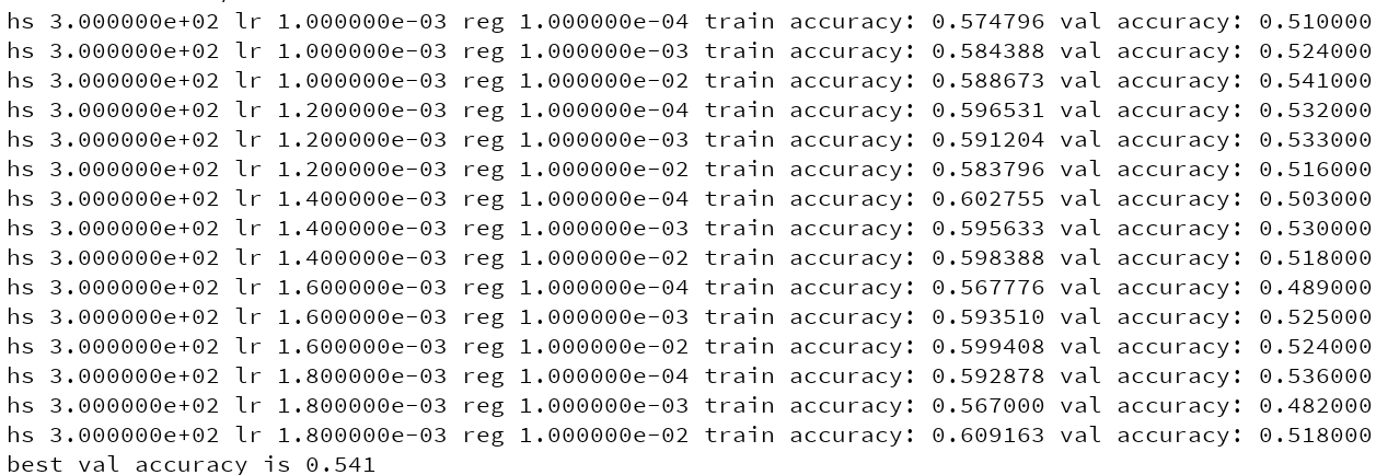
print('hs %e lr %e reg %e train accuracy: %f val accuracy: %f' % (hs, lr, reg, train_acc, val_acc))
print('best val accuracy is '+ str(best_acc))
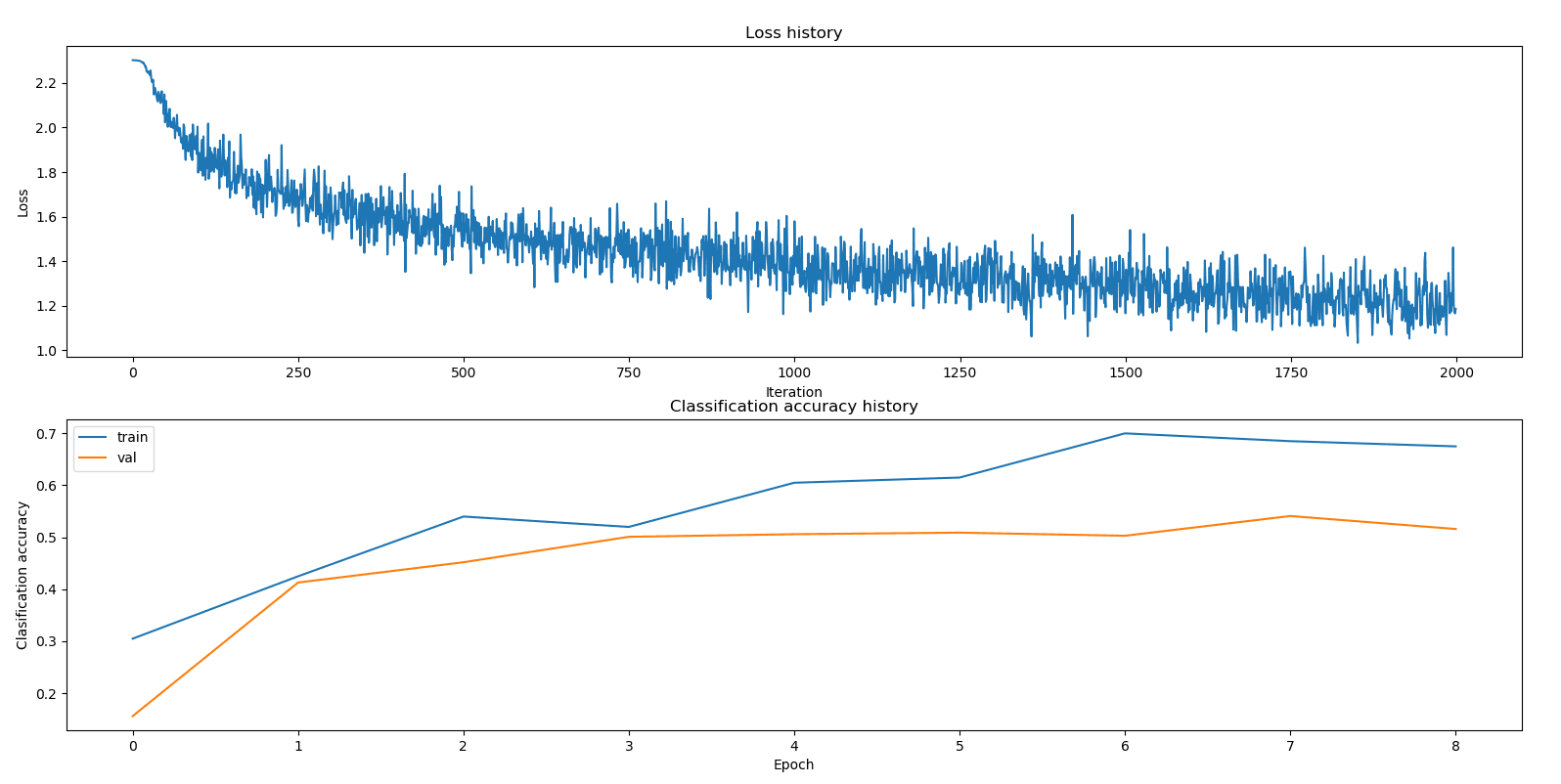
# Plot the loss function and train / validation accuracies
plt.figure()
plt.subplot(2, 1, 1)
plt.plot(best_stats['loss_history'])
plt.title('Loss history')
plt.xlabel('Iteration')
plt.ylabel('Loss')
plt.subplot(2, 1, 2)
plt.plot(best_stats['train_acc_history'], label='train')
plt.plot(best_stats['val_acc_history'], label='val')
plt.title('Classification accuracy history')
plt.xlabel('Epoch')
plt.ylabel('Clasification accuracy')
plt.legend()
plt.show()
结果